Tutorial 5: Working with PBR Materials

In this tutorial, we are going to use RapidCompact CLI to process and optimize PBR- (Physically Based Rendering) materials in form of textures of an input mesh, as well as handling the PBR workflow in general and applying metallic and roughness values to our output meshes. Physically based rendering is a philosophy in computer graphics that seeks to render graphics in a way that accurately describes light behaviour similar to the real world. Many PBR pipelines have the simulation of photorealism as their goal, however the state-of-the-art PBR approach for real-time applications cannot make practical use of all theoretical implementations yet. Even without all the benefits of a completely photo-realistic approach, the PBR concept still delivers more consistent and predictable rendering results than ever before in real-time graphics.

The materiality of 3D content will behave correctly in different lighting environments such as in Image Based Lighting scenarios.

PBR Basics

At first we will have a look at the basic principle of the PBR workflow for real-time graphics and how it can add value to 3D visualizations; real-time PBR materials mostly make use of three main areas of research taken from the general approach of physically-based rendering:

In the practical real-time use case, those areas are simplified and described as values from 0 to 1, or as greyscale RGB values from 0 to 255 per pixel, on a texture map.

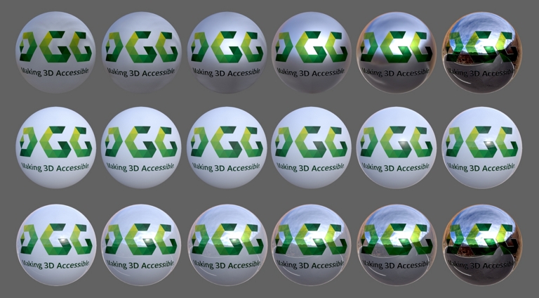
As a result, we distinguish between Metallic and Roughness maps, describing how metallic a material is (usually 1 or 0) and how light will be absorbed or reflected depending on the roughness or smoothness of a surface. In addition, the albedo map describes the color of diffused light. The following image shows the basic visual representations of metallic and roughness values in comparison:

Upper row (left to right): Roughness values of a metallic sphere from 1.0 to 0.0
Middle row (left to right): Roughness values of a non-metallic sphere from 1.0 to 0.0
Bottom row (left to right): Sphere with roughness 0.0, transitioning from non-metallic (0.0) to fully metallic (1.0)

Using the RapicCompact CLI to create PBR Materials from Values

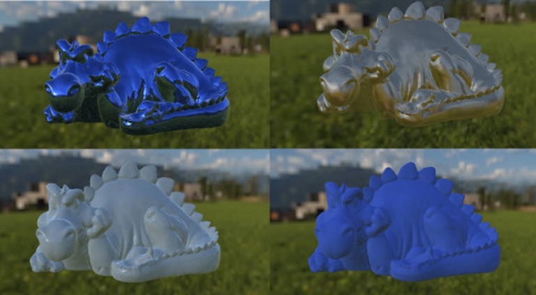
In this section we will apply basic PBR values to a mesh using the RapidCompact CLI. To get started, just download the sample mesh here. We will create four different material versions for the model.

The example Model with the four custom PBR material values applied.
Top left to bottom right: Blue polished metal, white half-metal, white porcelain, blue rubber.

These materials are just examples which do not necessarily exactly represent the materiality of real objects. However, they illustrate well how the different values interact with each other. Further PBR material parameters for real-world materials such as gold, copper or chrome, can be found here.

For achieving the different materials we have two options:

1.) Writing a config file and entering the different PBR values for each material

2.) Directly adding the values as a part of the CLI command itself

For method 1), just type the following command and write the file into your desired directory:

      rpdx --write_config
	 

After that simply open the config in an editor and find the following lines:

	   
     "material:defaultBaseColor": "1 1 1",
    

     "material:defaultMetallic": 0.2,
	 

     "material:defaultRoughness": 0.4,
    

Replace these standard values with one out of the following chart corresponding to the four sample materials:

We will now decimate the mesh to a sample count of 5000 faces and output it in the glTF format with the new materiality applied. Run the following command with the config file in place:

	rpdx -i dragon.obj --duplicate -d f:5000 -u -b -e dragon.gltf
	

For method 2.), simply ignore the config creation and use the these additonal commands between the baking command (-b) and the export (-e):

	-s material:defaultBaseColor "1 1 1" -s material:defaultMetallic 1.0 -s material:defaultRoughness 0.0
	

PBR Materials from Texture Maps

A more advanced approach to display PBR materials can be achieved by using Texture Maps instead of simple values. The different material properties can be stored in pixels as described in the first section.

The RapidCompact CLI will handle all PBR Texture Map Inputs and is able to convert multiple maps into one UV Atlas. In addition, the glTF formats Roughness/metallic and occlusion Textures will be stored in the respective RGB channels of the Texture file (Red=occlusion; Green=roughness; Blue=metallic)

To illustrate these functions we will go through the whole process of optimizing a mesh with several PBR Texture Maps applied and also cover real time web visualization in a PBR shading environment.

First of all we need the input mesh to start with, it can be downloaded here.

As you can see the file consists of a .gltf and .bin file with four different maps applied.

As a next step, we will create a compact glTF 3D Model for Web presentation purposes. In order to achieve that, we simply have to get our config file ready and then execute our optimization as a command in the RapidCompact CLI. At first, we will simply create a config file with the following command:

     rpdx --write_config

In order to create the best possible visual outcome while still reducing the file size significantly, some values can be altered. In this case, the most important changes are the file format change for the normal map in addition to the setup of the sample count for the baking process, which enhances the quality of the output normal map quite significantly. To compensate the increase of size due to the chosen png format, we can set the resolution of most maps to 1024, as RapidCompact already exploits the available UV atlas space quite efficiently. In the following we will replace some settings of the default config file with custom optimized settings for the example model:

After the config file is set up and in place, we can go on by simply typing in the following command in the RapidCompact CLI:

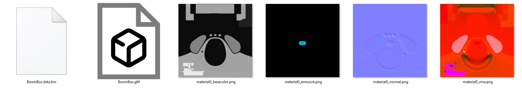
     rpdx -i BoomBox.gltf --duplicate -d f:50% -u -b -e Output/BoomBox_compact.gltf

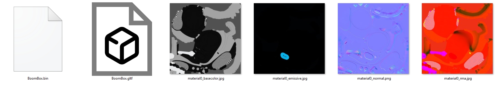
The resulting output files should now look like this:

The four maps are preserved and share one newly created UV Atlas. The Occlusion, Metallic and Roughness Texture Maps were rebaked into the respective RGB channels (so-called RMA) into one light-weight jpg file.

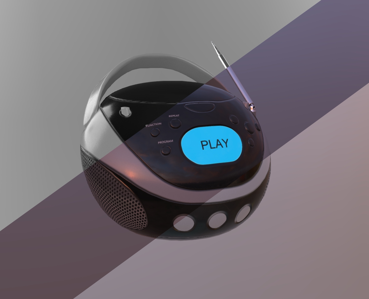
To further ease the handling of the model, we can simply output a single, self-contained .glb file instead of .gltf. The result will only be about 1MB in size, which is roughly 10x smaller then the input file, and you'll be able to directly view it in Windows 10 (using the mixed reality viewer, or inside applications such as MS Office), for example. If desired, rendered thumbnail images of the new model can be directly created with the RapicCompact CLI. The respective Tutorial can be found here.

In addition, the compact glTF model can be exported as a Web-ready HTML5 viewer, using the following command:

        rpdx -i BoomBox.gltf --duplicate -d f:50% -u -b -w web
    

To have a look at the result in 3D, you can either embed the Web container into your site, for example as an HTML iframe, or zip and upload the web directory to any Web server that will deliver it as static HTML content. The result should look similar to this version:

Tutorial 5: Working with PBR Materials